A histogram of instantaneous intensities emerging from the solar model
The four equations of stellar structure are all first-order differential
equations.
Each requires one boundary condition for a solution.
Two of these conditions are straightforward:
For the radial position r(m), r = 0 at m = 0.
For the luminosity l(m), l = 0 at m = 0.
Values of these quantities anywhere else in the model, but particularly at
surface R* = r(M) and
L* = l(M), are part of the solution.
The state variables ρ, P, and/or T are not known at the center, but presumably reach small values nearly indistiguishable from zero at the surface. But how 'indistinguishable' from zero are they and how important are the actual values?
1. Central Expansions
While the central boundary conditions may be straightforward, sometimes
numerical solutions are sensitive to how conditions behave at the center.
As far as material in the star is concerned, the center is no different
from any neighboring location.
We cannot apply the strict condition that gradients are zero at the center,
because that would over-specify the problem and very likely result in
the pressure dropping to zero before the density, or vice-versa.
But, near the center we can expand the primary dependent variables in terms of central values to reset the boundary to just outside the center:
r(m) = (3m/4πρc)1/3
l(m) = εcm
P(m) = Pc − (4π/3)1/3 (G/2)
ρc4/3 m2/3
T(m) = Tc + (Tc/Pc)
∇ ΔP ,
where ∇ is either ∇rad or ∇ad depending
on radiative or convective.
2. Surface Expansions
Radiative
Consider the radiative logarithmic gradient near the
surface:
∇rad = (3κP / 16πacGT 4) (L/M) ,
where we have assumed that the luminosity and mass have their total values.
Now write the opacity κ as
κ =
κo ρ n T −s ,
a form meant to describe the sort-of power-law opacities on either side of
the opacity peak at about 40,000 K.
Assuming an ideal gas, converting density to pressure gives
κ =
κo P n T −n −s .
We may then write the gradient as:
P ndP = (16πacGM / 3κoL) T n+s+3dT.
Integrating:
P n+1 = [(n + 1) / (n + s + 4)] (16πacGM / 3κoL) T n+s+4 [(1 − (To/T) n+s+4] / [(1 − (Po/P) n+1] .
For positive (e.g. Kramer's: 1, 3.5) or even zero (e.g. electron scattering: 0,0) values of n and s, clearly the actual values of To, Po are quickly overwhelmed, so the radiative zero boundary condition is adequate. Trouble arises when T < 104, and s becomes sufficiently negative as to make n + s + 4 ≤ 0. However, in those circumstances convection is also present near the surface, so the radiative gradient does not apply anyway.
Convective
As has been said before, the exact manner whereby flux carried by convection
is converted into radiation at or near the surface has significant effect on
a stellar interior (at least on the scale that we can observe in the Sun).
The asymptotic approach of the temperature-pressure gradient to adiabaticity
in the interior depends on details of the heat exchange taking place in the
moving material.
In addition, there are observational effects not present in any one-dimensional
model.
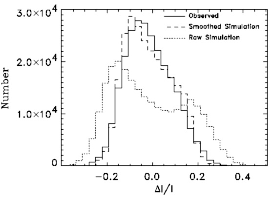
Consider the following graph from Stein's web page:
A histogram of instantaneous intensities emerging from the solar model
The raw simulation is double-peaked, with a contrast ratio between rising, hot, granules and sinking, cool, inter-granular material of ≈30%.
Now think about a star where we do not resolve granules, and see only the mean spectrum. About half the area is 30% brighter than the other half. The averaged intensity is then about 15% 'too bright' for the area; e.g. the spectrum we observe is weighted toward the hot granules. In effect, we are 'missing' 15% of the area. If we know the luminosity accurately and measure the effective temperature spectroscopically, we will think we are dealing with a hotter, smaller star than is really out there. A 15% error in area corresponds to a 7% error in radius, which is observable. We have very little knowledge of granule contrast ratios in other stars.
Nevertheless, we continue to use mixing-length theory.
Today's modelers use detailed grids of atmosphere calculations (e.g. those
of Kurucz, still the industry standard) to compute surface boundary expansions
for computation.
Kurucz models penetrate to relatively pure adiabatic conditions, so a grid
of T(P) curves as a function of depth may be accessed as the
calculation proceeds.
Atmospheres are usually tabulated according to effective temperature and
surface gravity, which can be converted into a grid over luminosity and
radius for a given mass.
One does not know L, R in advance, but at any stage of the
calculation one may assume values and see if they work.
Schemes abound for making corrections in the right direction.