Outline

4. Equation of State and Related Descriptions

4.4D. Fermi-Dirac statisitics

Elementary statistical mechanics leads to the following expression for the number of particles of species i in phase-space volume d ³r d ³p :

n_i(p) d ³r d ³p = (d ³r d ³p / h³) ∑ _j g_j {e ^{[−μ_i + ε_j + ε(p)] / kT} ± 1}⁻¹ .

ε_j = mc ²
ε(p) = mc ² {[1 + (p/mc)² ]^1/2 − 1}
v(p) = ∂ε/∂p = (p/m) [1 + (p/mc)² ]^−1/2
P = (1/3) ∫ n(p) pv dp .

Individual Fermi particles have g = 2 and the ±-sign reverting to +. With isotropy we have

n(p) dp = 2 (4πp²dp / h³) {e ^{[−μ + mc 2 + ε(p)] / kT} + 1}⁻¹ /cm³.

a. Complete degeneracy
Consider the 'exponential' part of the distribution, F(ε) ≡ {e ^{[ε − (μ − mc 2)] / kT} + 1}⁻¹.
As T → 0, F(ε) → 1 for ε > μ − mc ², and F(ε) → 0 for ε < μ − mc ².
We define the Fermi energy ε_F ≡ μ − mc ², or conversely μ = ε_F + mc ².
To find how these quantities depend on number density, let x ≡ p/mc, and consider the scaled Fermi momentum x_F that corresponds to ε_F through the ε(p) relation above. Now integrate the total density over momenta as

n = (8π/h³) ∫_o^p_F p²dp = 8π(mc/h)³ ∫_o^x_F x²dx = (8π/3) (mc/h)³ x_F³.

Substituting values for electrons gives n_e = 5.865×10²⁹ x_F³.

Carrying out the pressure integral gives

P = (8π/3) (mc/h)³ mc² ∫_o^x_F x⁴ (1 + x²)^−1/2 dx ≡ A f (x_F)
A = (π/3) (mc/h)³ mc² = 6.002×10²² dyne/cm² for electrons,
f (x_F) = x_F (2x_F² − 3) (1 + x_F²)^1/2 + 3sinh⁻¹x_F .

A similar expression may be written for the internal energy E(x_F).

These expressions cover the range from non-relativistic to relativistic. Converting x_F to n_e and then to ρ via n_e = ρN_A/μ_e gives

P_e = 1.004×10¹³ (ρ/μ_e)^5/3 in the non-relativistic limit, and
P_e = 1.243×10¹⁵ (ρ/μ_e)^4/3 in the relativistic limit (relativistic effects become important at about ρ/μ_e = 10⁶ ).

b. White dwarfs
At this point in their discussion, H&K briefly discuss the application to white dwarfs, referring to an admittedly approximate constant-density model. We could attempt to apply our 2-layer model with slightly more accurate results. A properly integrated polytropic model results in the classical Chandrasekhar relativistic limit

M_c = 1.456 (2/μ_e)² M_o ,

where M_o is the mass of the Sun.

c. Partial degeneracy
As one raises the temperature at any one density, the degeneracy becomes partial in the neighborhood of kT ≈ ε_F. For electrons, this transition occurs at

ρ/μ_e ≈ 6×10⁻⁹ T ^3/2 non-relativistic,
ρ/μ_e ≈ 5×10⁻²⁴ T ³ relativistic (the cross-over is at about T = 10¹⁰, ρ/μ_e = 10⁶ ).

A good model must treat partial degeneracy for densities within a factor of 10 on either side of this boundary. In the past, modelers have used various power-law expansions or some graded combination of degenerate/non-degenerate limits in the boundary regime, but today they use either pre-prepared tables or direct integration.

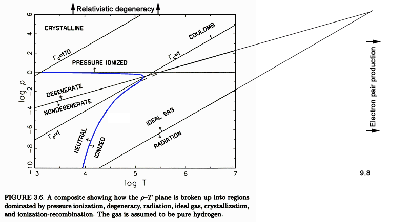
Below is H&K's figure showing state regimes on the ρ,T plane.